Maya Building Generator

Introduction

This project was created during my postgraduate degree, starting as a bonus objective but slowly evolved into its own standalone tool. Because of it’s origins and deadlines the project is ad hoc rather than general purpose. My goals are to experiment and explore procedural modeling practices using python in Autodesk Maya.

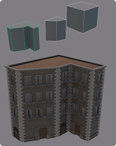
Starting with simple primitives modeled by the user the tool should automatically create detailed buildings, following the exact shape and dimensions of those primitives. In these images you can see some of the shapes I used throughout the process to stress and test additions to the code along with the resulting building on the bottom.

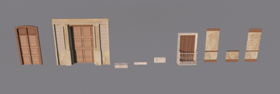
To achieve this I’ll use the help of kits to create the basic pieces and handle everything else in code. I modeled a modest kit for testing and the next step is to figure out where those pieces go in code. Let’s start with the windows, this should be easy, just loop over the height and width of each face, placing windows as you go. The trouble starts with finding the exact coordinates to place each window. To do this, I’ll implement a sampling function that uses bilinear interpolation to get the right positions along each side of the building.

Sampling Function

Let’s start by defining the inputs and outputs of this function.
As input this function must take parametric coordinates of a given quadrilateral face,

Input: (s, t)

and as output it must return the 3D world-space coordinates that correspond to our inputs

Output: (𝑥, 𝑦, 𝑧)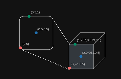

You can think of our s & t coordinates like the UVs used for texturing. When working with UVs we cut and flatten complex shapes into a 1x1 square. When we draw on the square our drawing is mapped from 2D relative coordinates on the UVs to 3D spatial coordinates on the model.

The 2D coordinate represents a percent of the surface, starting at 0 and ending at 1. So no matter the shape or size of the quad is (0,0) will always be the bottom left and (1,1) will always be the top right.

It’s important to note that unlike UVs, our coordinates are not used for texturing and do not need to be manually unwrapped since they represent a simple quad.

Using parametric coordinates as arguments makes it easy to turn a theoretical position into a 3D coordinate. Take a door for example, if I want to place a door in the center-bottom of a wall I can just use the ST coordinates (0.5, 0) as arguments. The function will return the world space coordinates (x,y,z) where we need to put our model, taking into account the translation, dimensions, shear, and rotation of the wall.

Placing rows or columns of objects, for example when distributing windows is also easy and would look something like this:

for(i in range(NumColumns)):
    s = i/(NumColumns-1)
    t=0.5

    worldSpacePos = sample(s, t)

    placeObject(worldSpacePos)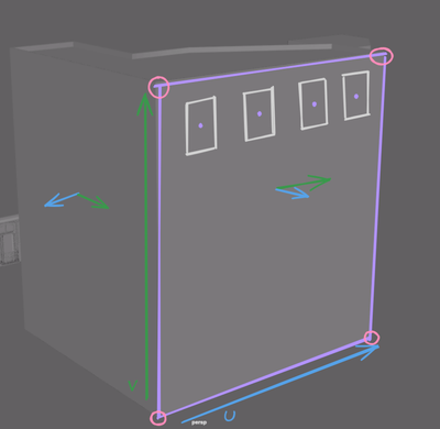

Bilinear Interpolation

Because our starting walls are simple linear quadrilaterals, I can use bilinear interpolation as the heart of the sampling function.

Linear interpolation is a simple but extremely useful mathematical concept to smoothly transition from one value to another. It works by taking to inputs and a bias. When you increase the bias the strength of one value goes up and the other goes down. Bilinear interpolation is when we perform this process in two dimensions.

For two dimensions we’ll need two biases, using our two s & t coordinates. For our four values to interpolate between we use our four corner coordinates.

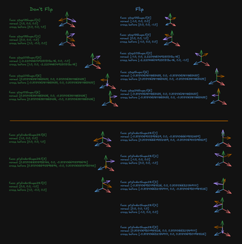
Bilinear interpolation provides the perfect solution for this problem, but with a very important condition. Bilinear interpolation only works if the points are consistently ordered when passed to the function. If the order is reversed so is the output leading to doors on the roof and diagonal lines of windows running across the walls.

Tangent Alignment Sorting

I came up with several approaches to consistently order the face vertices, each one failing in some aspect until I ultimately designed what I’ll call the Tangent Alignment Approach. This method works by comparing the position of each vertex to the center.

Before jumping into the formula we’ll need to establish/calculate a few things first. Starting with the face tangent $\hat{T}$ where
$\hat{T} = \hat{N} \times \hat{Y}$ and $\hat{Y} = (0,1,0).$

Next we need to compute the center point $C$ which we can get by averaging out all the vertex positions.
$\vec{C} = \frac{1}{n} \sum_{i=1}^n \vec{P}_i$
The math for this looks unnecessarily complicated, but the process is simple and can be more simply expressed through pseudo code.

total=0

for(position in vertexPositions):
    total+=position
total/len(vertexPositions)

Finally we compute a direction vector from the center of the face to each vertex.
$\hat{P}_d = \frac{\vec{P}-\vec{C}}{|\vec{P}-\vec{C}|}$

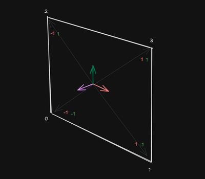
Now that we have all the components we can build the function
$f(\vec{P}) = ( sign(\hat{P}_d \cdot \hat{T}), sign(\hat{P}_d \cdot \hat{Y}))$

This is where it’s all leading up to, now we can assign the point order based on the output of this function.

$f(\vec{P}_1) = (-1, -1)$
$f(\vec{P}_2) = ( 1, -1)$
$f(\vec{P}_3) = (-1, 1)$
$f(\vec{P}_4) = (1, 1)$

This means that if the result of our function for a given point $\vec{P}$ is $(-1,-1)$ then that point will be sorted first. $(1,-1)$ second, and so on.

With this the sampling function is complete and can be used to create the rest of the project.

Kit Distribution

As stated previously the tool uses user built models and places them on each wall of the building. It starts by splitting the input primitive into conceptual pieces. The walls and roofs are identified based on the cross product between their face normal and $Y$ then processed based on their independent logic.

Walls

Walls start by gathering important data such as normals, tangents, and bounds as well as sorting the corner vertices. It then executes logic to populate each component of the building: windows, trims, doors, etc.

This logic uses the face normal as well as the sampling function’s output to construct a 4x4 transform matrix which is used to translate objects to their correct position, rotation, and scale. Each component has its own logic, but they all follow the same pattern: Source geometry is chosen, duplicated, and transformed by the aforementioned matrix.

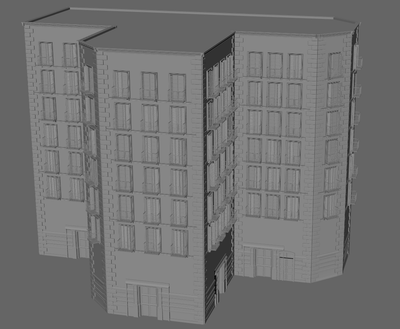
Windows are copied into grids, doors are placed at semi-random intervals on the bottom floor, and bricks are baked into stacks before being instanced onto the wall edges. The primitive is also being modified, the tool extrudes the roof, booleans gaps for windows, configures shaders, and scales trims into place (making sure to inversely scale the uvs to avoid distortion).

Each component has its own logic, but they share a similar structure.

Reference

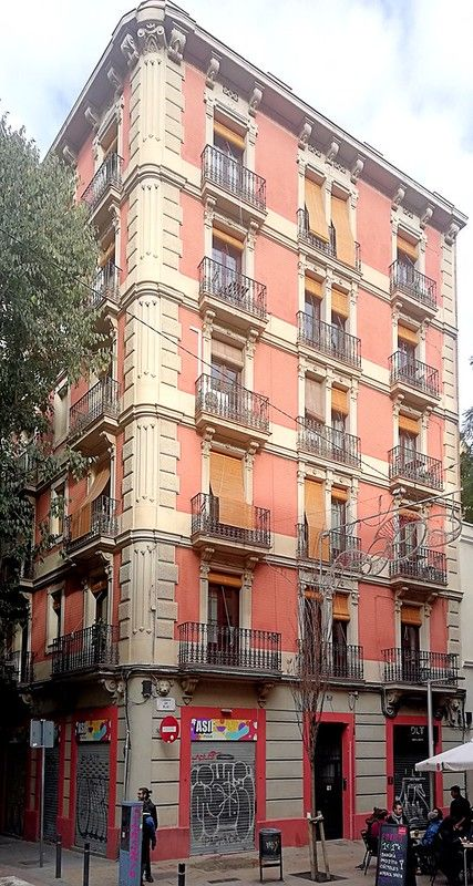
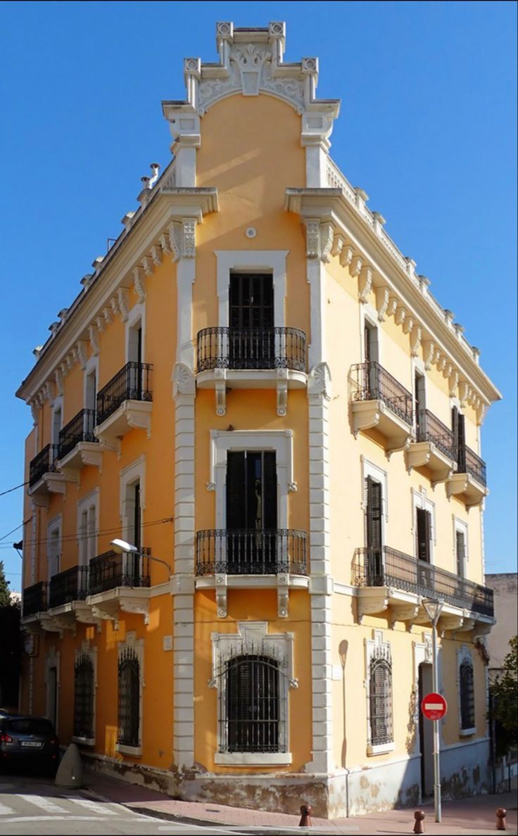
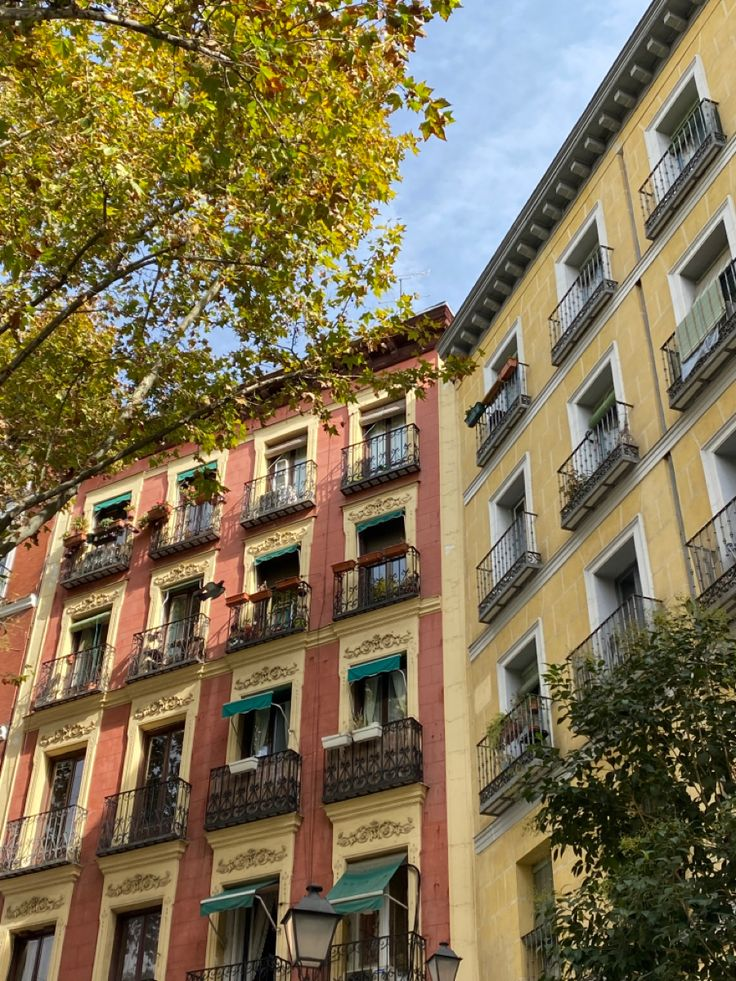
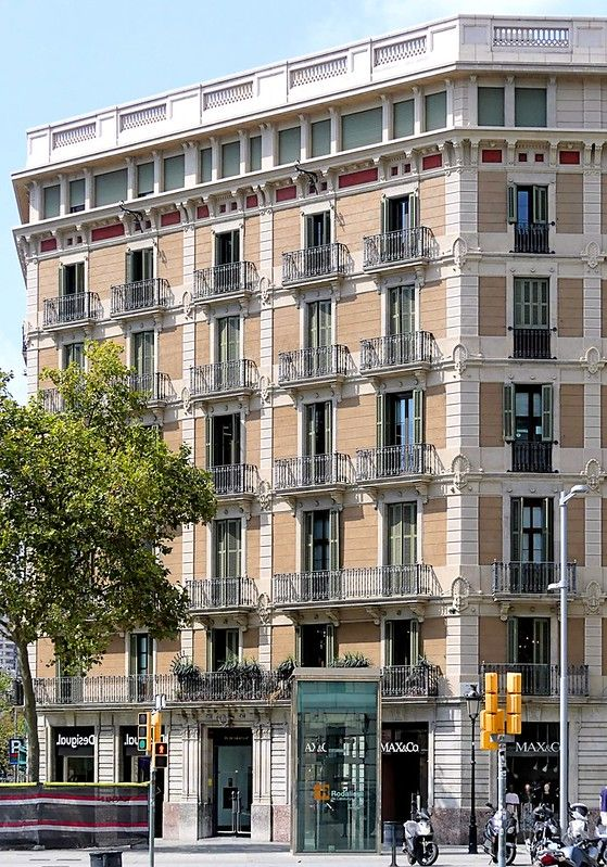
The style of architecture was directly inspired by Barcelona, Spain. I gathered reference, finding what made these buildings similar and different, noticing styles of trims, usage of balconies on windows, and bricks on each corner.

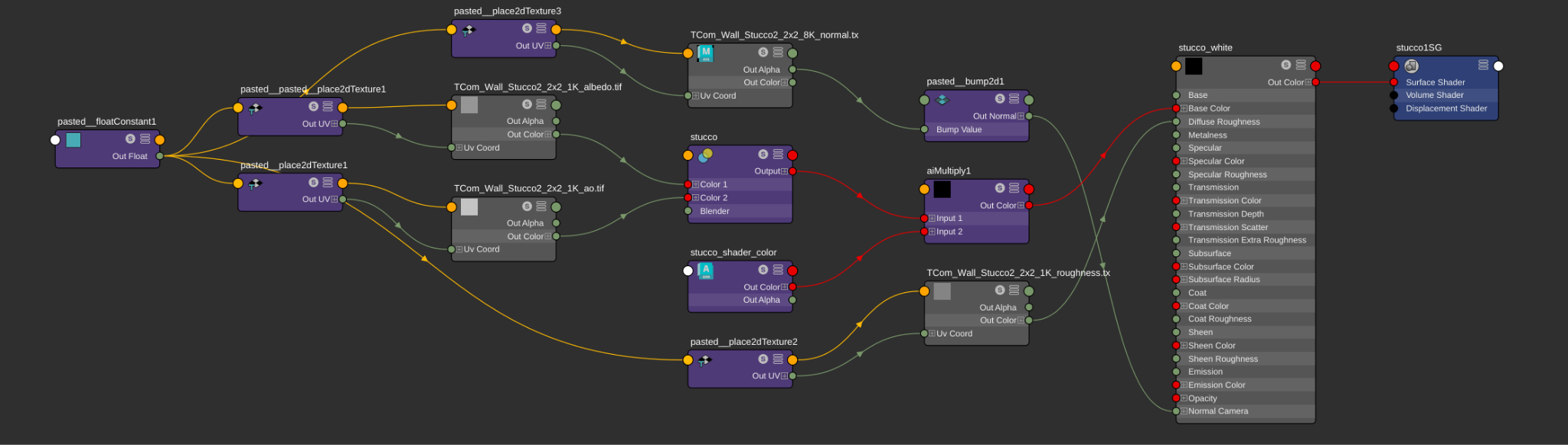
Shaders

I built several shaders, reading attributes set by the code to define properties such as color. Each building receives semi-random attribute values, making each building visually distinct in color and geometry. The project is made up of more than 13 shaders for the various models, such as the one pictured below.

Optimization

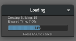
I spent a lot of time considering and modifying for execution speed. I built a loading bar, so I could monitor the progress and benchmark different optimization techniques. I used instancing to reduce the memory footprint of heavily repeated objects, prebaking/combining heavy geometry processes for reuse, and batching boolean operations into a single action.

Along with Maya’s slow copy operation, I encountered massive performance hits after several copies. While software like Houdini can easily handle millions of instanced models, Maya slows to a crawl after a couple hundred. Based on observation Maya seems to exponentially degrade in performance the more objects are in a scene. I found that by merging meshes together Maya could handle the same amount of polygons with much better performance.

Self Reflection & Future Work

Overall, I’m satisfied with the result, given the time I had, although there are several areas I’d look to for improvement.

Throughout the project I mostly focused on solving the technical challenges involved, slightly neglecting the visual result. Because of time constraints and limited modeling skills I made only a few variations of the asset kit models. For future work the addition of a more varied and advanced kit could greatly improve the visual product.

This project was created ad hoc and as a result was mostly tailored for that particular use case. Because of its specialization additionally user control and generalization would further the tool’s usefulness.

I managed great strides in performance from where the project started, but the generation is still slow. Whether this is a limitation of the platform or my techniques is not clear, but additional work is needed.

Overall, unless I want to punish myself, I’m not keen on doing more procedural modeling in Autodesk Maya. The software’s design doesn’t lend itself to this type of project and while I enjoyed the mathematics and problem-solving I didn’t enjoy the instability and performance issues along the way.